The number of digital buyers has been increasing for the last few decades, and even the COVID-19 pandemic hasn’t interrupted this trend. In fact, lockdowns and social distancing policies only fuelled a spike in online shopping. In 2020, the number of digital shoppers exceeded two billion people, and e-retail sales surpassed $4.2 trillion worldwide.
Experts forecast that the global e-commerce market will expand by $1 trillion by 2025. It means that more new e-retailers will enter the market, and competition among market players will become more intense.
What e-retailers should do to keep their companies afloat in the long run? They should revisit and update their pricing policies to hit two birds with one stone: maximize profitability and win customer loyalty.
How can they do it? One of the ways they can do it is to leverage reinforcement learning for dynamic pricing.
Today, we will talk about reinforcement learning, dynamic pricing, and how it helps retailers keep pace with price movements.
The concept of dynamic pricing
Before we dive into the topic, let’s define the term dynamic pricing and explain how this strategy differs from static pricing.
In a static pricing strategy, the price remains constant over a long period of time. In dynamic pricing, the price goes up and down depending on the demand (and other market factors) at a given time.
When dynamic pricing is applied, the system changes the price of products and services in real-time to maximize the retailer’s income and improve the key performance indicators, such as average transaction value and conversion rate.
How does the system find the “optimal price”? The system monitors the changes in market positions and adjusts the price based on the following parameters:
-
Previous and current price of the product
-
Previous and current competitors’ prices
-
Changes in consumer preferences
-
Changes in target audience’s shopping behavior
-
Timing (time of the day, the season of the year, etc.)
How can dynamic pricing help retailers?
The key benefit of dynamic pricing is that it allows retailers to analyze the market trends in a quick way and determine “the right price” for the product.
What is “the right price”? It’s the price that satisfies customers at the given point of time yet allows retailers to get the most bang for their buck.
Who can benefit from dynamic pricing?
Dynamic pricing strategy is not a new thing. Airlines, car rental companies, hotels, train companies, and concert venues have been using dynamic pricing strategies for years to adjust their businesses to changing market conditions and get ahead of the competition.
Uber and dynamic pricing model
Uber is one of those companies that apply a dynamic pricing model. If you use Uber for a while, you know that the cost of your ride depends not just on the distance of your trip but also on weather conditions, the current demand level, and other factors.
Let’s consider an example. Imagine that the normal fare of your Uber trip “Home – Airport” is $30. If you travel to the airport on Friday at rush hour (high demand time), you will have to pay a higher price (around $40). And if it is raining heavily, the cost of your trip will increase even more – you will have to pay around $50 to get to the airport on time. That’s what dynamic pricing is all about – as an Uber user, you can agree to pay more and get served immediately, or you can wait until the prices go down.
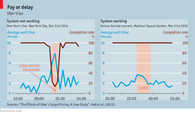
Even though most customers have negative attitudes toward surge pricing and higher-than-normal rates, the dynamic pricing system proved to be highly effective. The experts from Economist compared the average time it takes to get an Uber in case of demand surge a) when the system IS NOT working and b) when the system IS working.

Image source: economist.com
They found out that the average wait time increases drastically when the system is NOT working, and the completion rate drops. And when the system IS working, the situation is different. The completion rate is 100%, and the average wait time doesn’t increase that much, even at the busiest hours. It means that overall customer satisfaction remains high, and the company keeps completing orders and earning money without any significant disruptions.
Why should you consider using dynamic pricing for your e-commerce business?
If you want to stay competitive in an ever-changing market, you should use a flexible pricing model. You should adjust prices as quickly as new trends emerge.
If you opt for a dynamic pricing strategy, you will get a competitive advantage. It will be easy for you to define a peak season and a low season for a product. You will know when exactly you should lower the price to boost sales and when you can increase prices without risking losing your customers.
Researchers state that dynamic pricing can improve revenues and profits by up to 8% and 25%, respectively. However, it all depends on the size of the market and the number of transactions. The bigger the market you operate in, the greater the opportunity for profit maximization you can enjoy.
Another great benefit of implementing a dynamic pricing strategy is that it allows you to gain in-depth market insights. You can better understand changes in consumer behavior and make more informed strategic decisions in the short and long run.
Dynamic pricing and e-commerce world: challenges and opportunities
Even though dynamic pricing has lots of advantages, it also has one specific drawback – you never know for sure how consumers will respond to the price change. When the price jumps up, there is always a risk that you will lose the loyalty of your clients.
Above, we’ve considered an example where the cost of an Uber trip went from $30 to $50 because of high demand and bad weather conditions. That’s an example of a dynamic price change that most customers can tolerate.
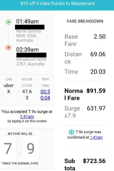
However, there are other situations in which the use of a dynamic pricing strategy results in a more significant price surge. For instance, in 2016, Sydney Uber prices surged by 800% on New Year’s Eve.

Image source: smh.com.au
That was the situation that negatively affected Uber’s reputation. Many users, who overpaid for their trips, sworn off to never use the app again.
In other words, using dynamic pricing, you can’t overcome the uncertainty of customer response. To solve this problem, you need to use sales data more wisely.
What is “sales data”? Sales data can be defines as a sequence of data points (prices) indexed in time order. It includes information about product prices, revenues, and other variables that affect sales (inventory, prices set by competitors, technology trends, fashion trends, seasonality, etc.)
Sales data is input. It’s information the merchants need to design an effective dynamic pricing software.
We should emphasize the fact that measuring real-life agent performance is a challenging task. For this reason, further, we will consider an artificial example rather than a real-life example.
What kind of sales forecasting model will we use? We will opt for a model where the market state is considered an “input” and estimated sales – “outputs”. The price will be considered as an individual independent variable that acts as the input of the system.
How will we train agents to find an optimal pricing strategy? We will use a complex approach. We will apply advanced machine learning methods and exploit big data (sales data) for time series forecasting.
Prognostication models: two alternative approaches to find the right solution and build a winning pricing strategy
We can use two methods to define a pricing strategy: a simple one and a complex one.
Let’s start with a simple one – one-step optimization approach. That’s how this forecasting model works: we set various prices (high prices, low prices, and any random prices) and analyze how they influence our profitability levels.
What more should we know about a predictive model? We can define this model as a non-parametric model in which data distribution cannot be determined in terms of a finite set of parameters. It means that we can’t apply gradient-based optimization techniques to this model.
Instead, we can encode continuous attributes in discrete attributes and turn them into countable numbers – the possible prices. It will allow us to pick the price associated with the highest potential income or achieve another objective.
What are the pros of this method? When we use this method, we avoid falling into the “local minima” trap.
What are the cons of this method? This method is a greedy one. It does allow us to maximize income right here and right now, but it doesn’t help to accumulate income. In plain English, this approach can help e-retailers increase their income in the short run but will not help them maximize their profit in the long run.
What is the best alternative approach to dynamic pricing? What method can help merchants to keep the greedy algorithm under control? The best alternative solution here is reinforcement learning (RL).
RL is capable of identifying the relationship between the successive pricing stages. What does it mean? RL is non-greedy for current sales. Yet, it’s greedy for cumulative gain.
For instance, reinforcement learning can define the timestamp where retailers need to lower prices and get lower income in the short run to get higher income once the market conditions change.
The basics of reinforcement learning
What is reinforcement learning? It’s a machine learning training method that draws on rewarding desired behaviors. Software developers use RL to write algorithms that aim at maximizing cumulative reward. These algorithms are applied to agents that explore the unknown environment.
Now you may be wondering how we can describe the environment. We need to apply Markov Decision Process (MDP), a mathematical framework that represents reinforcement learning environments. That’s a framework where an agent may role-play different scenarios and affect the results.
Further, we will use a finite horizon MDP. Here is a formula:
p (s', r ∣ s, a) = P (St=s', Rt= r | St – 1 = s, At - 1 = a)
∑ s ′ ∈S ∑ r∈S p (s', r ∣ s, a) = 1, where s ∈ S, a ∈ A
Here are the elements of the formula:
-
S state space (finite set)
-
An action space (finite set)
-
R reward space (a subset of real numbers, finite set)
-
p dynamics function (defines the dynamics of the MDP)
Now you may be wondering how agents interconnect with the environment (MDP). There is one interaction per each time point: t = 0, 1, 2, etc.
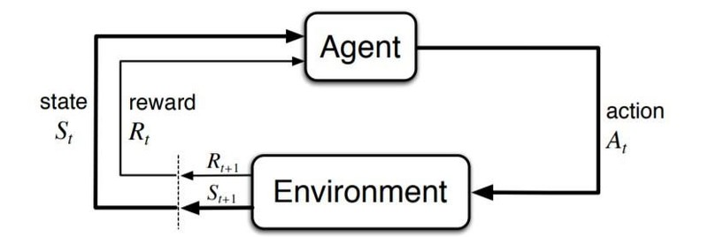
That’s how we can describe this process: the agent takes a step (an action “a”), the action itself is derived from “s” (current market conditions). The MDP picks the action “a” and reacts with a reward “r” – further, it randomly moves into a new state, “s’”, and gives a decision-maker a corresponding reward “R”.
Here is how this sequence looks like:
S0,A0,R1,S1,A1,R2,S2,A2,R3,...
Take a glimpse at the following visualization of agent environment interaction in an MDP.

Image source: towardsdatascience.com
As we have already mentioned, the key objective of reinforcement learning is to level up the cumulative income that the agent ultimately expects to receive (reward hypothesis). Now we should define a return as a reward function. If we consider episodic tasks (the tasks that terminate), the function will be the following:
Gt = Rt + 1 + Rt + 2 + Rt + 3 + ... + RT
Now let’s take a look at the function of policy, which describes the process of MDP.
π(a∣s) = P (At=a∣St=s)
Further, we should define two functions: the first one is state-value, and the second one is action-value. These functions demonstrate the amount of cumulative income a retailer can get in the state defines as “s” while taking “a”, a designated action:
vπ(s) = Eπ[Gt∣St = s]
qπ(s,a) = Eπ [Gt∣St=s, At = a]
According to this theory, there is a minimum of one policy defined as “optimal” in the given environment. This policy holds the highest value regarding all possible states. And that’s a key point of the RL algorithm – it always strives to get closer to an optimal solution.
Application of reinforcement learning and solution of dynamic pricing challenges
When we talk about dynamic pricing and its benefits, we expect an agent to analyze current market trends and find an optimal pricing solution. And what do we consider “actions” associated with RL? Actions are a set of all possible prices, states, and market conditions, excluding the product’s current price.
In most cases, it’s challenging to sample train reinforcement learning agents with goals for real-world tasks. It takes agents too much time and effort to collect lots of sales data.
Besides, agents face the exploration-exploitation trade-off – a fundamental dilemma of learning more about the world by trying things out. The dilemma is between making decisions and getting the results close to what you expect (“exploitation”) and choosing something you aren’t sure about, and possibly learning more (“exploration”). Sometimes, it makes an agent act in ways that result in significant financial loss for the company.
To save time and money, agents need to opt for an alternative solution. They should utilize simulated data rather than real-world data. The only challenging task here is to recreate transitions that show how states change one another. Well, it’s not that easy to simulate changing market conditions properly, but there is the only way to make this strategy work.
Tabular Q-learning
In a nutshell, Tabular Q-learning is a model-free reinforcement learning algorithm. Take a look at its basic formula:
Q*(s,a) = maxπ Eπ [Gt∣St = s, At = a]
Knowing this formula and the values of the designated actions, agents can get an optimal pricing solution. Basically, that can be any policy defined as a “greedy” one. Here is an updated formula to use:
Q (St,At)←Q (St,At)+α [Rt+1 + γ*maxa Q (St,a) − Q(St,At)]
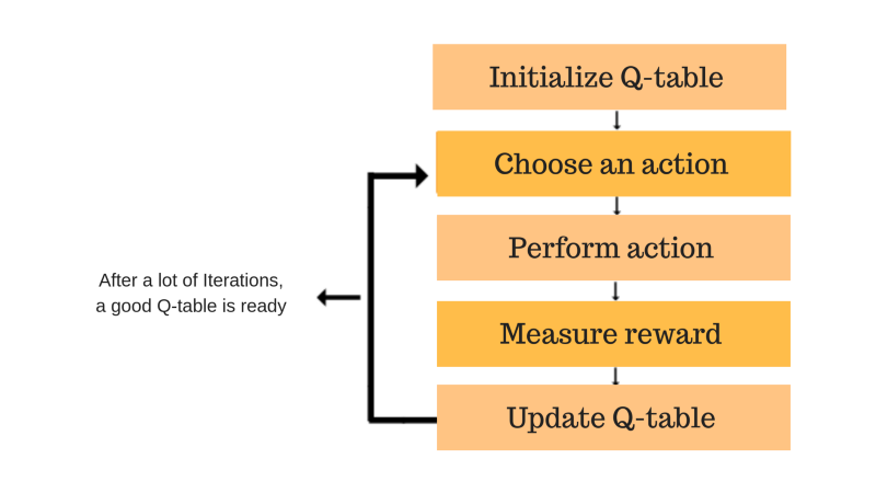
The Q-function uses the Bellman equation and takes two inputs: state and action. The process of values updating can be described as iterative. As the agent updates the Q-values in the Q-function, they can get better approximations.

Image source: freecodecamp.org
The first thing you should do to run this algorithm is to chop data – transform continuous variables into a discrete form. As you can see, the name of this algorithm includes the word “tabular”. It means that the system store all action values in one enormously-big-in-size table.
Naturally, the more features and variables are added to the table, the more the training time and memory usage are extended. It’s the reason why Tabular Q-learning does not work for complex environments.
Deep Q-network
The next algorithm we consider is the deep Q-network (DQN). This algorithm is pretty similar to the Q-learning algorithm we have discussed above. However, there is one significant difference. In contrast to Q-learning, DQN utilizes a parameterized value function optimization. This machine-learning algorithm applies ANNs, artificial neural networks, which work as approximators.
Q (s,a;θ) ≈ Q*(s,a)
What are the benefits of a deep Q-network? It can work with high-dimensional data, including images. Besides, this algorithm proved to be off-policy sample efficient. DQN allows us to use one chosen sample multiple times and take advantage of experience replay.
Policy Gradients
Now let’s talk about the algorithm that lies at the core of policy gradients. This algorithm implies a totally different approach to get an optimal price. Policy gradients do not focus on finding the best values action, and it doesn’t demonstrate greedy behavior. Instead, this machine learning algorithm directly parameterizes and optimizes a policy.
π (a∣s,θ) = P (At=a∣St=s, θt=θ)
Policy gradients perform way better than a greedy agent, but still, it cannot be compared with deep Q-network in terms of effectiveness. If you decide to leverage policy gradients instead of DQN, you will need to use more episodes samples to update the policy parameter θ.
In conclusion
You can be sure that if you use reinforcement learning in your e-commerce business, you will overcome dynamic pricing challenges. You will maximize your profit and get ahead of the competition.
Just keep in mind that if you implement this strategy, you should be transparent with your target audience about your practices. You should inform people about the possible price changes upfront to prevent misunderstandings and preserve the loyalty of your customers.

